Introduction

This contribution presents a significantly enhanced and reworked version of an abstract presented at the AIUCD at Sapienza University, Rome in 2017 . The field this contribution is centered in is stemmatology or more precisely computational and theoretical stemmatology. Stemmatology itself is the science of reconstructing the genealogy of text versions belonging to the same tradition (that is work) based on surviving text versions in order to obtain a text as close as possible in form to how the authorial original might have looked (compare , . Stemmatology is thus a philological sub-discipline primarily concerned with works of ancient and medieval authors that had been transmitted in hand writing. Graphically and theoretically, the main framework with which stemmata are being modelled and described is graph theory, more specifically, nodes (or vertices) symbolize text versions while edges symbolize genealogical relations, that is copy processes. Before briefly introducing the history of the field with a focus on computation and graphics in order to subsequently describe the two main target problems tackled in this paper, the reader may arm herself/himself with an understanding of the some very recurrent basic stemmatological terms which will be used otherwise unexplained throughout the rest of the article, for all of them compare also :

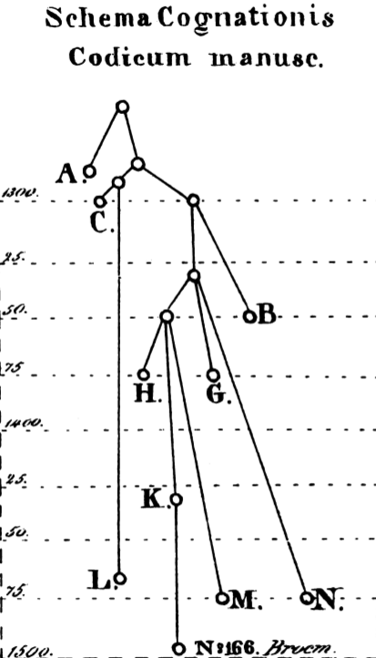
stemma or stemma codicum: literally a genealogical tree of the codices ( , 190) is a reconstuction of the copy history of one and the same work (for instance of all versions of Caesar's De Bello Gallico). In Figure 1, such a stemma is shown. Note, that it contains two different sets of nodes: such which are mapped to an extant text and such for which the text versions need to be reconstructed bottom-up so as to ultimately arrive at the text of root (should this not be present in one of the extant witnesses).
tradition (or textual tradition): other than the common usage of the term, in stemmatology tradition refers to all versions of a text in which it has been transmitted.
textual witness: A (textual) witness is one concrete version (or manifestation) of a text of a tradition. For stemmata, witnesses are what a node symbolizes, not manuscripts (since those are rather the physical embodiment of the witness and since they can carry other texts alongside the witness of the actual tradition).
reading: a reading is a short piece of text varying between manuscripts ( , 162), where one can think of the tradition as an alignment with one column per witness and a row holding the aligned corresponding readings.
vorlage: Vorlage is a loanword from German which refers to the model of a copy, thus if one imagine a scribe copying the text of one manuscript A into a new manuscript B, then A is the vorlage of B. The German plural is vorlagen, the English one can be vorlages.
archetype: an archetype of a tradition is usually the witness that coincides with the root of a stemma or a further reconstruction based on it. It needs to be differentiated from the original, which is assumed to be lost for most actual cases of application of stemmatology. With the original lost, the reconstruction closest to the original is that text which can be reconstructed on the basis of all extant versions and their stemma (and if one will an additional step of changing obvious fallacies etc.). Often it is graph technically the latest common ancestor of all surviving witnesses (sometimes one node above). Its text is the archetype and as such, if to be reconstructed, the best-we-can-do reconstruction.
edition: an edition is essentially a print version of a work. Firstly, version here entails a reworking rather than variation through copy edits and errors. Secondly, there is a difference between born-printed texts and born-handwritten texts when it comes to editions. A print edition of a born-handwritten text can contain for instance a) one retyped (transcribed) version of the text from one particular manuscript or b) a reconstructed archetypical text or c) multiple versions of the text and others more, which born-printed editions do not map to. Especially for c) there are many different scholarly edition types that have come into existence and with them different methods to derive them, the most famous of which is probably a so-called critical edition often featuring a base text to be read with superscript anchors relating to a (often heavy) footnote apparatus noting all variants.

Brief History of Stemmatology and its Assets in Computation

The beginnings of stemmatology depend on its definition. For the author, the occurrence of modern stemmatology is bound to a key event: the invention of the printing press. This ground-breaking invention brought with it a fundamental change to the way (and of course numbers) in which texts were transmitted. Namely, a printed book features the exact same text as many times as it was printed. A manually copied work, due to the imperfection and variation of human concentration and copy skill (but also philological activity) differed in each exemplar. Furthermore, with years of transmission smaller copy errors, idiosyncratic translations and small edits (for instance modernizing a text) could accumulate and lead to quite different versions in different regions. Thus, only with the invention of print, a key question gradually came into focus: given a variety of versions in different manuscripts, which of these should be printed? For the author, this question is the birth-place of modern stemmatology. The discipline investigating variation in textual transmission is much older (although presumably itself a product of the introduction of writing) and is called textual criticism. One of the first textual critics could have been Zenodotus of Alexandria , , who investigated the differences between the versions of Homeric works already roughly 2300 years ago.

While prima facie the early printers tended to choose manuscripts in their vicinity , , philologists gradually started discussing ever more the genealogy of manuscripts as a tool to identify good extant texts and (for instance in case that text is far removed from the prospective original) a reasonable way of reconstructing bottom-up an archetypical text. In 1737 Bengel proclaimed a perfect edition of the New Testament would propose a classification of the codices for their genealogical relations ( , 9) and not even one hundred years later, in 1827, what has been identified as the first stemma in a modern sense by ( , 62) is published for Swedish law texts by Carl Johan Schlyter, see .

First stemma in a modern sense, 1827, identified as such by (Timpanaro 2005, p. 62).

The next most important two events are the summarizing formulation of a method of deriving a stemma mechanically from the surviving witnesses attributed to Karl Lachmann (see also ) and the fundamental criticism at the method by Joseph Bédier in 1928 who proposed an editing paradigm which would only determine a best manuscript by some reasoning but not construct or draw graphical equivalents of the copy history. Bédiers criticism was existential and had large effects, one of which was the reaction of Paul Maas in 1937 who claimed that despite not sharing Bédiers preoccupations on the genealogical method of Lachmann in general, there was a phenomenon which was irremediable: contamination. In section , this will be explained in detail. Some years later, Pasquali and Pieraccioni talk about 'vertical' and 'horizontal' transmission distinguishing contamination from inheritance. The phenomenon has a slight implication that the Lachmannian method of stemmatology be more appropriate for the latter. recently argued that precisely such factors should be clearly reflected when applying certain digital methodology.

Already in the early days of computation, stemmatological tasks have been conducted by computer programs . While in the beginning the computer was thought to be capable of helping only with some more unsubtle subtasks ( , 72), continuously growing hardware capacities finally led to the complete automation of the stemmatological task. With the 1990ies an influx of bio-informatic software was noticable and dominated the field until the time of publication of this article, but genuinely stemmatological algorithms and procedures independent of the use of bio-informatical software have appeared lately, for instance , , .

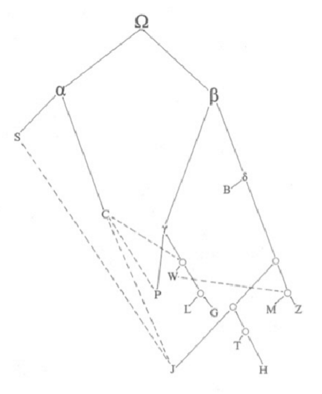
Example of a (typical) philolocigal stemma, here by (Lundström 1989) reprinted in (Silvas, Anna M. 2013).

Transfer of software generated for one field to another one is often correlated with a cumbersome process of adaptation and accommodation. As for stemmatology, this shall be exemplified by the properties of the graphical representation of the stemma since it is very closely correlated with the formal model one can apply to it, overtly or covertly. shows some classical stemma as they appear in the prefaces of editions. As ( , 509) mention, the preferred graph theoretical model used for stemmata in the literature adhering rather to the uncontaminated tradition type is a Directed Acyclic Graph (DAG) or in more common terms tree. As one can immediately see from the previous figure, this is not the case for some classical stemmata, where philologists included various nodes with an indegree > 1 in order to indicate that contamination happened. Bio-informatically generated stemmata further are marked by a graphical focus on the leafs (which are the only labelled nodes) and by being unrooted and thus undirected. Hence, they, too are no DAG, but an unrooted tree. This implies the question what model one can apply to a stemma satisfying the needs of classical philology without dissecting it into open and closed or imposing a threshold on how much assumed contamination must be present to keep a stemmatic hypothesis satisfactory. Since the focus of this discipline is on the most uncorrupted and thereby authentic text version, hence on the root (compare ), we can conclude that temporal order of the tree or directedness and rootedness are utterly important. Yet at the same time, some way has to be found to maintain the possibility of indegrees >1. The result is not only a graph, but a specialized type of graph which can be modelled in different ways one of which is the subject of the next sections.

Contamination

( , 47) define contamination as The confluence of readings from more than one exemplar, ( , 15) explains contamination as The entering into a manuscript of readings that derive from a source other than its exemplar. As mentioned in the abstract, the term is an umbrella term for different phenomena. To begin with, mention three types of contamination, extra-stemmatic or extra-archetypical ( , 134) contamination refers to variants in extant manuscripts which come from lost exemplars (or such lost exemplars from branches between the original and the archetype). ( , 108) estimates that for the average tradition no more than 27% of the witnesses have presumably come down to us. Extra-stemmatic contamination must be one of the most prevalent types of contamination given these large numbers of witness loss (see for a general account of causes of manuscript loss). The second contamination type is simultaneous contamination where simultaneously a scribe had two or more vorlagen and chose between variants of them for instance, this was one main vorlage and a secondary one which she/he consulted in case the main one was hardly readable, had a lacuna or was damaged. The third type, successive contamination refers to the type of text mixture where for instance the first half of a text is copied from one vorlage and the second half from another also known as exemplar shift. However, there are even more types of contamination, for instance contamination from memorized text. More importantly, medieval manuscripts may contain some text in the margins or between the lines, which partly note or discuss alternative variants.

Towards a universal stemmatic model

Few explicit models other than DAGs have been outlined for stemmata. None of them maintains two philological requirements at the same time. Firstly, the temporal order of a stemma graph, secondly, the requirement of having two types of nodes, extant ones and (at least partly) reconstructed ones. However, in philological stemmata, we do see that even though their underlying models are hardly ever formulated mathematically, the existing models and especially the DAG could only be taken as a basis for a fraction of them. Thus, we try to generalize the DAG in a way that would allow the new model(s) to be postulated as implicit model underlying any philological stemmatic depiction. One advantage would be that if this succeeded, any philological stemma would become more readily accessible as stemma comparationis for computation.

The main idea of the current proposal is inspired by existing graph types which are more complex in their definition than simple graph types such as DAGs. They require some additional elements or constraints. Such graphs are for instance multiple edge class graphs as defined by or multi layer graphs, as defined in .

The simplest way of modelling what could lie behind the graphics of classical stemmatology maintains the time-ordered DAG defined through a set {V, E, r} and expands it by a second set of edges E’ the members of which may not belong to E. Those edges would be termed contamination edges. The model would be applicable to all philological stemmata which use two different line types (e.g. normal and dashed) such as the stemma of Lundström above, see .

Let S be a stemma graph with S={V, E, E', r}

with V the vertex (or node) set entailing the vertices v_i ∈ V and with E a set of pairs from V: E⊆{{u,v}: u,v ∈ V, u≠v}

and with E' another set of pairs from V: E '⊆{{u,v}: u,v ∈ V , u ≠ v, {u,v}∉ E}

and r is a distinguished node root.

The logic behind S is that for any copy c (which would be labeled v_i), we assume there to be one main vorlage v_m and any number of secondary ones v_s1, v_s2, ... Secondary vorlagen must be older than c and different from v_m, there is no necessary hierarchy between them. From this follows that an edge {v_m , c} ∈ E and for each secondary vorlage an edge {v_si, c} ∈ E' exists. Empirically it appears conclusive that a scribe most of the cases chose a main exemplar since switching too often could be impractical. This model can hold well for simultaneous or successive contamination. For extra-stemmatic and extra-archetypical contamination, in this model, we would assume additional vertices which have at least one secondary (contaminatory) edge but no primary (main vorlage) edge. Thus, we would include them into the stemma as hypothetical nodes (for which only the contamination inducing portions might [have to] be reconstructed). Consequently, the term extra-stemmatic would loose some of its adequacy, but in general, since philological stemmata often tend to represent those vertices, rather something like extra-reconstructional or extra-full-reconstructional than literally extra-stemmatic may describe the phenomenon. Any other type of contamination could be accommodated as well by simply typing the edges and allowing multiple types for one edge.

Getting more Complex – Back to the (Oral) Roots

Furthermore, in case we deal with an oral origin of a work, traditional stemmata are complicated by the fact that variation that has sprung from oral transmission is partly different from written-copy variation compare , . While this can be mapped somehow on the edge type, one of its consequences needs another model-theoretical intervention: roots. The text of an orally transmitted epic is different every time it is being performed and any first written manifestation springs from a dictation or writing-down event , . As one can imagine, popular plays such as the Odyssey can have manifested in written multiple times independently and thus all bare a slightly different (oral variation type) text. The work of Zenodotus in comparing Homeric versions was thus surely somehow different from that of philologists of the post-print age and the model of transmission he could have had in mind presumably somehow different from a modern stemma by this necessity. For such a work, basically from the different first manifestations, copies may have sprung in the usual way, one could thus assume two or more independent DAGs or stemma graphs, but due to contamination these would mix with each other ever more, the further down one proceeded in the tree. For consolidating this with the model, either one could allow multiple roots or one could assume one ultimate oral root from which then in the second generation all written manifestations (from the oral) sprang. Even a later back and forth of written and oral transmission as attested or supposed variously, (see for instance ) could be accommodated by such an extension where necessarily some nodes would be of an oral type. Lastly, the phenomenon of strata in a manuscript as alluded to for instance by could be taken into account for a general stemmatic model by defining a node as a sequence of successive states and requiring edges to dock onto node states. This is a kind of maximally general model which could be more fit to express the high complexity of stemmatology in many respects and yet graphically it would still look strikingly similar to a simple DAG. Leaving this as narrated theoretical allusion, coming back to the stemma graph S, we realize that this was consistent only with philological graphical stemmata which have no more than two linetypes but there are several, which have three.

A Refined Model for Contamination

In case two main types of contamination would be distinguished, as is presumably intended by graphical stemmata through displaying three line types (e.g. normal, dashed and dotted), things get more complicated. If we deal with extra-stemmatic contamination in the same way as above and assume that successive and simultaneous contamination are the two types to be displayed differently, then one could deal with successive contamination by assuming that there is still one witness contributing the largest part to any copy c. Only in case of truly the same number of contributions could one allow multiple main edges belonging to E. This however would be a model theoretical problem in the sense the graph constituted only by E would no longer be a DAG which could mean loosing some analytical benefits. For that reason, here we introduce an assumption which relaxes that situation albeit at the cost of loosing comparability between different traditions through a differently set parameter. The reasoning why one can presumably always find only one single main vorlage builds on a structural observation. Witness size can be counted in different ways and different granularities: by pages, by chapters, by words, by letters. The level(s) on which we count is our additional parameter. In case more than one witness contribute exactly the same to a copy in a completely unambiguous case, they would have to contribute the same number of pages, chapters, words and letters. This however is highly unlikely if there is free independent text in all parts of the witness. In other words, given different options for counting the size of the contribution to a copy, one could theoretically always find quantitative arguments to support intuitive prioritization of one vorlage if only slightly (by more letters or more words). But this would be, so my guess, relevant only in few cases anyway.

If we thus define one vorlage as global main vorlage v_gm, then in any successive or previous part, where it is not the principal vorlage, it can still be used for simultaneous contamination, just not for both at the same time and likewise all partial main vorlagen v_pm cannot be secondary vorlagen v_ps for the portion where they are the principal vorlage. Thus, we can define two edge sets E'_sim and E'_succ for simultaneous and succesive contamination. For each copy c, we define possible ancestry to be composed of one main (successive) vorlage v_gm, entailing an edge {v_gm, c} ∈ E. Additionally there can be edges indicating successive contamination for each vorlage of another section of c ( v_gm can be vorlage to discontinuous sections) {v_pm, c} with v_pm ≠ v_gm, all ∈ E'_succ. Finally, we can have edges indicating simultaneous contamination. These are of three qualities. First, there may be witnesses not serving as a main vorlage to any part of c. Those simply form edges {v_i,c}∈ E'_sim.

Secondly, the global main vorlage was used for simultaneous contamination in any of the further sections, then we add another edge {v_gm, c} to E'_sim. And lastly, if any of the other main vorlagen for the sections were used for simultaneous contamination, this constitutes an edge {v_pm, c} ∈ E'_sim. Thus we allow multiple edges from one to another node. And in fact, we do find philological stemmata or partial stemmata with this number of edge types (see for instance the stemma in , 48). Moreover, the classical stemmata where we find two edge types seem most prevalent, the ones where a third edge type is present exist, but more than three edge types, I conjecture to be rare. Not always do two additional edge types map to successive and simultaneous contamination. Finally, some graphical depictions draw the same edge type for contamination and main edges pointing to and allowing uncertainty – as outlined above, we assume that if enough evidence on the text was available one could resolve such uncertainty and therefore not further operate with so-modelled graphical stemmata. It must likewise be said that two other types of stemmata which are often given are not touched upon by our considerations: stemmata variantii ( , 52) for words and partial stemmata.

There is an important restriction on S, whether we define it with one or two additional edge sets: E must constitute a DAG, that is no cycles are allowed in E, any vertex v_i has an indegree(E,v_i)=1 and there is a certain number of nodes with outdegree(E,v_i)=0. The graph is of course directed. In order to maintain this, we need a second assumption for the model, namely that ultimately no two nodes are generated at the exact same time, but that even among descendents of the same main ancestor, the time of completion differs.

Counting Contamination Scenarios

The statements that stemmatics is not useful if contamination is present in its most extreme fashion is one which we can now theoretically and quantitatively assess. In order to do that, we count and confront the number of possible scenarios of stemmata involving contamination with those which do not and try to align the result as quantitative argument with the philological discussion.

If we model a stemma tree as S with one additional edge set, we can ask, for a tree of n nodes, how many contamination edges are maximally possible. The number of edges for any tree is (n–1). Thinking of the possible place to insert the first contamination edge of E', we have apriori n possible sources and (n–1) possible target positions if selfloops are disallowed, which they are. By differentiating source and target, we imply direction. But, younger nodes can just be contaminated by older ones, which is why we have to divide n (n–1) by 2. This is so because when taking all n possible sources combining them with each of the (n–1) possible targets, then every undirected edge is generated twice, once with n_i being the source and n_j, i≠ j being target and once the opposite where n_j is source and n_i target. If we assume a different point in time of generation for all nodes, even siblings, then only one of the two generated edges can be a valid one, namely that where source is the node with the earlier point in time of generation whether this be n_i or n_j. (n(n-1))/2 would be the number of insertible edges. But, we would still have to subtract the existing (n–1) edges of E arriving at a formula for all places, a first contamination edge could be inserted as: (n (n–1)/2) – (n–1). Now, for any number z of contamination edges to be inserted, we seek the formula for all possible contamination scenarios. We know that wherever of the (n (n–1)/2)–(n–1) possible places we place the first one, the second one can be placed at exactly one place less so as to not coincide with the first one. More generally, (i–1) places are already occupied if i is the ordinal index of the actual contamination edge to be inserted, for the second edge i=2, for the third 3 etc. Thus (n (n–1)/2) – (n–1) – (i–1) positions are possible at each step. Now the question is how to count all different contamination scenarios and an obvious assumption would be multiplication. For each scenario of insertion of the first contamination edge, we can insert a second one at (n (n–1)/2) – (n–1) – 1 places. But, if we would leave it at that and multiply (n (n–1)/2) – (n–1) – (i–1)) with (n (n–1)/2) – (n–1) – 1), we would overgenerate since the sequence of contamination edges is unmeaningful in our context. So while (n (n–1)/2)–(n–1)) gives us all possible places for a first contamination edge and (n (n–1)/2) – (n–1) – 1) gives us the places for a second one, when spelling out all scenarios the case that we have chosen any specific possible first contamination edge e_iand with it a second one e_jwill essentially be equal to the scenario where we have first chosen e_jand then e_i. So in this case we would have to divide the result by 2 but more generally we would for each sequence e_i,e_{j ,}e_k … generate all possible permutations and thus we have to divide by z! (which for 2 is 2). Then, we can answer the question for how many contamination scenarios C can we have for a tree with n nodes if we want to insert exactly z contamination edges by the formula:

(1) C(z)=(Π_i=1..z (n(n–1)/2 – (n-1) – (i–1))/z!

The maximum number of z is of course, as outlined above n(n–1)/2 – (n-1) which implies exactly one scenario – a scenario of extremely promiscuous witnesses where any possible contamination edge is realized –, warranting that Π_{i=1..(n(n–1)/2 – (n-1))} (n(n–1)/2 – (n-1) – (i–1)) = z!. If we look more closely, we see that very regularly the exact middle between 1 and (n(n–1)/2 – (n-1) is the place with the maximal number of possible contamination scenarios, which could be interesting when talking about large amounts of contamination being plausible in philology. If these amounts would be so large that virtually all manuscripts are contaminated by all possible contamination sources, then the contamination hypothesis would simply be as probable as the one without contamination.

Now in order to know how many scenarios are possible for contamination at all, when we don't know z to confront the full complexity of contaminated versus uncontaminated traditions, we can sum all contamination scenarios of all possible values of z. Then, the maximum possible number of differing contamination scenarios C_max with a tree of n nodes under the model is:

(2) C_max =Σ _z=1.._{(n(n–1)/2 – (n-1))}C(z)

Ultimately, we will also know how many trees including contamination are possible at all by multiplying with the number of all possible trees for n nodes:

(3) n⁽ⁿ ^– ¹⁾ * C_max

The problem is one based on graphs and many equivalent problems have been identified already in the literature, for instance the number of possible labeled planar graphs, compare the OEIS sequence number A288266 and sources therein, for instance . Ultimately, the numbers we generate are intimately related with Pascal's triangle by reproducing its rows for each n when incrementing z (but with the restriction that we do not allow z to be 0 and thus loose the first number). Abstracting towards a more easily expressed but more abstract formula, we see that C(z) equals C(C(n-1,2),z) and that C_max equals 2^{((n(n–1))/2)} – 1, compare OEIS sequences A084546 and A006125 (A126883).

Turning to an assessment of the philological debate, we now confront the number of scenarios for contaminated traditions (according to (3)) with the number of scenarios for uncontaminated traditions (as n^(n–1)) for any tree of size |V|=n up to 10 in a table. The table shows the factor with which the number for uncontaminated tradition scenarios would have to be multiplied to equal the one for open tradition scenarios, which equals C_max, the number of all possible contamination scenarios per single tree since n^(n–1) is a factor in (3).

Tree size	No Contamination	Contaminated Tradition	Factor
1	1	1	1
2	2	14	7
3	9	567	63
4	64	65472	1023
5	625	20479375	32767
6	7776	16307446176	2097151
7	117649	31581162845295	268435455
8	2097152	144115188073758720	68719476735
9	43046721	1514571848868095273151	35184372088831
10	1000000000	36028797018963967000000000	36028797018963967

Scenarios and factors

As one can see from the values, the numbers for contamination scenarios are much larger and in addition grow quicker which in terms of the philological debate would imply that contamination being present makes a specific stemmatic hypothesis mathematically a much weaker hypothesis.

At the same time at very low numbers of overall nodes, contamination implies moderately more complexity. For n=2, the contaminated traditions are only 7 times as complex as the uncontaminated ones where at 8 nodes they are already more than roughly 69 billion times as complex. Looking at the mere numbers, one can also read the table in a relativizing way: a contaminated tradition of a backbone tree with only 5 nodes is roughly half as complex as an uncontaminated one with 9. Then, rejecting stemmatics on the basis of complexity of contamination would be more consistent if one would also reject it for uncontaminated traditions of certain sizes.

One could argue that for different traditions, different amounts of contamination may seem likely and that only contamination below a certain amount could be dealt with. We tabulate anew this time with the tentative threshold for z = (n–1)/3 rounded up to the next integer. Thus threshold t gives the maximally allowed number of contamination edges (0 still excluded).

Tree size	Uncontaminated	t	Contaminated Traditions (t)	Factor
1	1	0	0	0
2	2	0	0	0
3	9	1	9	1
4	64	1	192	3
5	625	1	3750	6
6	7776	2	427680	55
7	117649	2	14117880	120
8	2097152	2	484442112	231
9	43046721	3	158498026722	3682
10	1000000000	3	7806000000000	7806

Scenarios and factors

Such an assumption heavily influences numbers and the added complexity of contaminated traditions is no more as astonishing as in the unconditioned case though still large at larger numbers of n.

In summary, this small and very theoretical counting exercise using a simple model that could lie behind many a philological stemma graph implies conditionals on a statement like contamination precludes stemmatology if one were to believe in it in this extreme form. Firstly, it depends on the estimated degree of contamination (as we have seen above where fewer scenarios were possible both at very mild and very large degrees of contamination), secondly on the overall size of the tree constituted by E, where smaller trees do not imply as severe a difference in complexity between contaminated and uncontaminated tradition scenarios as larger ones. To understand the true meaning of such statements or opinions as contamination precludes stemmatics one would have to investigate philological stemmata in more detail observing for up to how many witnesses do philologists empirically publish stemmata and how many nodes do these have. How many of them have 2 and how many 3 edge types. How are they judged by the community. Are factors such as time pressure and payment important in a decision on whether to edit in a Bedierian or Lachmannian fashion. Is there any empirical consensus among the community and is the community aware explicitly. And especially, how large is the amount of contamination that philologists include in their stemmata. For this purpose a database of stemmata where scholars could input a published stemma, the tradition, the graph encoded in some way distinguishing contamination and the publication would be utterly useful.

It is self-evident that contamination complicates stemma building in the first place and entails a localization of contaminatory processes increasing its complexity so that our quantitative argument reflects only an aspect of the implication of contamination. Hopefully it could however be shown nonetheless that unconditioned statements can entail contradictory implications which should be resolved as much as possible.

A final word to a computational realization of contamination models. Well, of course, using a model like the one outlined, a fallback to tree-generating software (such as bio-informatic one) without some adaptation would hardly be possible. There is a way of automatic exemplar shift detection and consequently, stemmata for different parts of a work can be produced, but simultaneous contamination is currently possible to assess automatically only if one abandons the temporal ordering altogether and generates for instance phylogenetic networks. However, here no real difference between uncontaminated and contaminated inheritance can be spotted. The here-outlined model for contamination allows to generate and maintain a backbone tree constituting E and then add contamination for instance by some post-processing scenario.

However the reception of all this, there is still hidden complexity, for instance in modelling different scribes (hands), redactions, different proportions of lost material in any one witness and developing even more complex contamination models. Doing this will enable rational comparisons and a larger throughput and capacity of evaluation of otherwise easily unreflectedly overread implications of different assumptions for those who are willing and able to use such tools and to adapt them if necessary.

Visualisation of contamination via an excursus on multiple languages

A problem of a similar magnitude as contamination and correlated with it is translation. Translation of a renowned work has some benefits, for instance a certainly less heavy creative workload. Translation is important in many textual traditions. By using evidence from manuscripts of the same textual tradition in other languages but also by introducing changes to the text required by the different grammatical set-up of languages contamination and translation are interrelated and both produce variation. We will exemplify visualisations which can be used to display either contamination or translation. In order to show how they can be applicable to translation as well, we use this phenomenon here although our toy tradition to be introduced is not contaminated.

Practically, various philological stemmata, for instance incorporate translation (using yet again different edge types). If one wanted to use a distance matrix based method to induce a genealogical hypothesis, translated texts would be a problem in the sense that words could be no more compared as simple strings to derive some similarity because even if a corresponding translation of a word was used, the surface form in both languages would differ and a simple metric such as Hamming asking if two items are the same would need a hidden meaning layer to operate. Another possibility would be the use of language independent structural elements such as the chapter sequence as used monolingualy by or the sequence of first appearances of named entities or other rather structural (for instance narrative) elements.

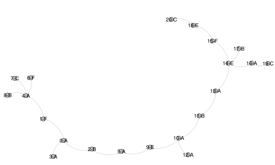
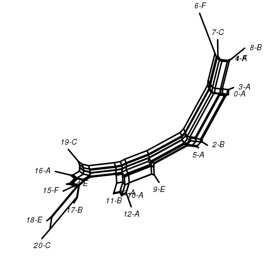
In order to know and compare with the true tree, we produce a toy tradition by introducing a root chapter sequence where each chapter is symbolized by one letter and then induce copying. Upon each copy slight changes can happen. Both sequences and copy processes are recorded. First, a randomization decides between one and four copies per generation and then proceeds for each copy. Translations outnumber again by randomization monolingual copies twice. Randomly the copy is assigned an ancestor from a previous generation and the copying starts. We suppose that translation, since it is a freer process than monolingual copying introduces more deletions, insertions, expansions (simply using two chapters for where the original sequence has one) and contractions (simply contracting two adjacent chapters into one new chapter) as well as transpositions on the level of chapters. We set the probability for all but transposition to 1% impressionistically and for transpositions to 2% in the monolingual copy case whereas we choose twice that probability for the cross-lingual case. The process ends when the size of the tree has grown to 20 and produces a tree, see . Finally, we produce a second flavour of the tradition and loose 4 chapter sequences, among them root.

This toy tradition is sufficient as a case that reflects data which probably has never but could be structured in the way it is (possibly through other processes and possibly not as historical tradition but as Wikipedia article versions or homeworks concerning similar topics copied from internet precedents etc.). In the following, we want to look at possibilities of visualisation and analysis for this toy tradition exemplifying what can be done with at least comparable data in the humanities.

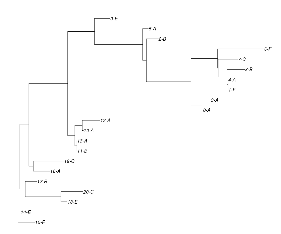
The true tree generated by our chapter sequence copy process. Root is 0-A. Letters mark languages.

NJ tree for the entire toy tradition, generated with R, package ape.

First, two methods from the realm of bio-informatics are being presented. The Neighbor Joining algorithm generates an unrooted phylogenetic tree and can be seen in . As one can see, it is retracing many of the relationships in the true tree albeit in the typical bifid manner. The root however is not distinguishable.

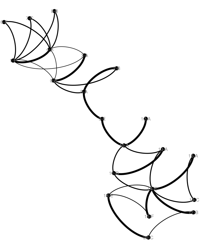
The second visualisation, see is a so-called NeighbourNet . This visualisation is applicable to displaying which sequence (or text) is close to which other and can thus be used to display contamination although a genealogical hypothesis is not immediately derivable. Again, the true relationships are captured by the general outline of the net. The third visualisation goes back to Minimum Spanning Trees (MST). MSTs depict only the surviving nodes and connect them to a tree which spans all nodes of the graph and on which the sum of edge weights (corresponding to the corresponding distance matrix field) is minimal given all such possible trees. Now, whenever there is one value in the matrix, which is the same in more than one field, theoretically more than one equally likely MST can exist . uses an implementation of method 1 as described there to generate all MSTs which we also use. In one further step, the algorithm counts all edges in all MSTs and creates a consensus graph with the edge weights corresponding to the number of MSTs that the edge was present in. Because of a quick combinatorial increase, already two or three instances of duplicate values in the underlying distance matrix can quickly lead to larger numbers of MSTs and we found a number of 1536 MSTs. has proved that all those MSTs must constitute a chain where neighbours differ only in one edge which is why despite this enormous number, the consensus MST features only 33 edges in all, where a tree would have 19 (n-1) and the weights show that the enormous number is truly a result of combination, see . This consensus MST could be used as a way to display contamination visually. In the case of translations it may help us find out which witnesses belong to the same redactions in case there have been multiple translations from and into the same language. Again the general typology reflects the true givens to a certain extent.

NeighbourNet generated with R package phangorn.

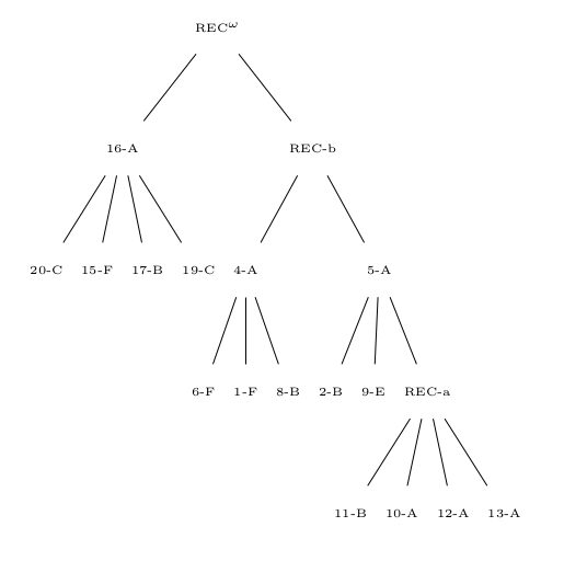
Lastly, an approach similar to the monolingual approach in produces editable LaTeX code as in (Hoenen 2016) and can be characterized as iterative clustering. Finding a way of representing contamination in this method would come even closer to philological habit, which is why we shortly introduce the method here. Instead of a bifid clustering, starting from the pairwise matrix of distances, all witnesses cluster which are below a certain threshold of distance (hence where they are very similar). There can be incompatible clusters which can be resolved merging them, as for phylogenetic networks in . The next step is to apply philological or linguistic knowledge by rules. For each tradition, the user can edit and compose these rules herself/himself. Here, we only simplistically sketch one that is based on our prior knowledge of A to be the source language:

If in a clustered group, there is only one manuscript of language A, it will be considered cluster root otherwise a lost A exemplar will be hypothesized.

Consensus MST — The network of edges present in 1536 MSTs, visualized with gephi. Edges by degree of thickness correspond to presence in all (1536), half (second thickest), a third or a quarter of the MSTs.

Extant manuscripts end up either as internodes or cluster root with this procedure. The next step consists of updating the matrix, which is a step similar to the concurrent steps in NJ or its predecessors. All clusters/groups are identified, named and a new empty pairwise distance matrix between them is set up. Every cluster will be represented by its root. Unchanged pairwise distances (in case either a cluster had only one member or in case root had been a present witness according to the rules) are then retrieved from the old matrix. The empty fields are filled by the average of distances of all with all group members of the two clusters. When all fields of the new distance matrix are filled, another round of clustering is executed. This happens iteratively until after a terminal clusterstep either there is only one group left uniting all previous roots or when only groups remain, which have one single member. Ultimate root is again generated according to the rules above. Since by this logic, an idiosyncratic text would get placed very high up the tree per se, since furthermore, the nodes closest to root in the actual stemma end up rather removed from the root, the outcome should be yet interpreted as unrooted (see ). While the other visualizations were either entirely bifid or produced no hypothetical nodes, this tree has both multifurcations and hypothetical nodes and offers manipulation through external rules. However, the accuracy seems inferior to the other methods, an update step closer to the NJ procedure taking into account different evolution rates could improve results. Groups such as (4,6,1,8) have come up and nodes close in the true tree appear mostly close here, too. Contamination could now be introduced in various ways in the latter procedure, for instance by detecting similarities among the textual versions across branches of the final outcome and introducing contamination edges where these are the strongest (until a certain threshold). This however should only be conducted if the results of the method are more reliable, which has to be further tested and developed. Be it this method or another to be developed, the technical possibility to produce graphs which are non-bifid and include hypothetical nodes exists. Furthermore, such a graph can be rooted and enriched by the display of contamination. All four visualisations display witness relations very differently; two of them are per se applicable to display contamination, all 4 to display translation.

Iterative cluster tree on the toy tradition with missing texts 3, 7, 14, 18 and 0, unrooted.

References

Amodio, Mark. 2004. Writing the Oral Tradition. Poetics of Orality and Literacy. Notre Dame, IN.: University of Notre Dame Press. http://www.loc.gov/catdir/toc/ecip052/2004023679.html.
Andrews, Tara L., and Caroline Macé. 2013. Beyond the Tree of Texts: Building an Empirical Model of Scribal Variation through Graph Analysis of Texts and Stemmas. Literary and Linguistic Computing 28 (4): 504–521. https://doi.org/10.1093/llc/fqt032.
Baez, Fernando. 2008. A Universal History of the Destruction of Books: From Ancient Sumer to Modern Iraq. New York: Atlas & Co.
Bandelt, Hans-Jürgen, and Andreas W. M. Dress. 1992. Split Decomposition: A New and Useful Approach to Phylogenetic Analysis of Distance Data. Molecular Phylogenetics and Evolution 1 (3): 242–52.
Bédier, Joseph. 1928. La Tradition Manuscrite Du ‘Lai de l’Ombre’: Réflexions Sur l’Art d’Éditer Les Anciens Textes. Romania 54 (214, 215-216): 161–96, 321–56.
Boden, Brigitte, Stephan Günnemann, Holger Hoffmann, and Thomas Seidl. 2012. Mining Coherent Subgraphs in Multi-Layer Graphs with Edge Labels. In Proceedings of the 18th ACM SIGKDD International Conference on Knowledge Discovery and Data Mining, 1258–1266. New York: ACM.
Bodirsky, Manuel, Clemens Gröpl, and Mihyun Kang. 2007. Generating Labeled Planar Graphs Uniformly at Random. Theoretical Computer Science 379 (3): 377–86.
Buzzoni, Marina, Eugenio Burgio, Martina Modena, and Samuela Simion. 2016. Open versus Closed Recensions (Pasquali): Pros and Cons of Some Methods for Computer-Assisted Stemmatology. Digital Scholarship in the Humanities 31 (3): 652–69.
Cameron, H. Don. 1987. The Upside-down Cladogram: Problems in Manuscript Affiliation. In Biological Metaphor and Cladistic Classification: An Interdisciplinary Approach, edited by H. M. Hoenigswald and L. F. Wiener, 227–42. Philadelphia, University of Pennsylvania Press.
Casson, Lionel. 2002. Bibliotheken in Der Antike. Düsseldorf: Artemis & Winkler.
Castellani, Arrigo E. 1957. Bédier Avait-Il Raison?: La Méthode de Lachmann Dans Les Éditions de Textes Du Moyen Age: Leçon Inaugurale Donnée à l’Université de Fribourg Le 2 Juin 1954. Fribourg: Éditions universitaires.
Cayley, Arthur. 1889. A Theorem on Trees. Quarterly Journal of Mathematics 23: 376–78.
Cisne, John L., Robert M. Ziomkowski, and Steven J Schwager. 2010. Mathematical Philology: Entropy Information in Refining Classical Texts’ Reconstruction, and Early Philologists’ Anticipation of Information Theory. PloS One 5 (1). https://doi.org/10.1371/journal.pone.0008661
Dearing, Vinton A. 1974. Principles and Practice of Textual Analysis. Oakland: University of California Press.
den Hollander, August. 2004. How Shock Waves Revealed Successive Contamination: A Cardiogram of Early Sixteenth-Century Printed Dutch Bibles. In Studies in Stemmatology II, edited by P. van Reenen, A. den Hollander and M. van Mulken, 99–112. Amsterdam: John Benjamins.
Ellison, John W. 1957. The Use of Electronic Computers in the Study of the Greek New Testament Text. Cambridge, MA: Harvard University.
Fazzo, Silvia. 2017. Lo Stemma Codicum Della Metafisica Di Aristotele. Revue d’Histoire Des Textes 12: 35–58.
Flight, Colin. 1990. How Many Stemmata? Manuscripta 34 (2): 122–28.
Flight, Colin. 1992. Stemmatic Theory and the Analysis of Complicated Traditions. Manuscripta 36 (1): 37–52.
Foley, John M. 2002. How to Read an Oral Poem. Urbana, IL: University of Illinois Press. http://www.oraltradition.org/hrop/.
Foley, John M. 2012. Oral Tradition and the Internet: Pathways of the Mind. Urbana, IL: University of Illinois Press. http://www.pathwaysproject.org/.
Fourquet, Jean. 1946. Le Paradoxe de Bédier. Mélanges 1945 (II): 1–46.
Greg, Walter W. 1927. The Calculus of Variants: An Essay on Textual Criticism. Oxford: Clarendon Press.
Haugen, Odd E. 2015. The Silva Portentosa of Stemmatology Bifurcation in the Recension of Old Norse Manuscripts. Digital Scholarship in the Humanities 31 (3): 594–610.
Hering, Wolfgang. 1967. Zweispaltige Stemmata. Philologus-Zeitschrift Für Antike Literatur Und Ihre Rezeption 111 (1–2): 170–85.
Hoenen, Armin. 2016. Das Erste Dynamische Stemma, Pionier Des Digitalen Zeitalters? In DHd 2016 Konferenzabstracts. http://dhd2016.de/boa.pdf
Hoenen, Armin. 2017. Beyond the Tree - a Theoretical Model of Contamination and a Software to Generate Multilingual Stemmata. In AIUCD, Book of Abstracts, 155–59. DOI 10.6092/unibo/amsacta/5885. http://amsacta.unibo.it/5885/#
Hoenen, Armin. 2018a. From Manuscripts to Archetypes through Iterative Clustering. In Proceedings of the 11th International Conference on Language Resources and Evaluation. LREC 2018. Miyazaki (Japan). http://www.lrec-conf.org/proceedings/lrec2018/summaries/314.html
Hoenen, Armin. 2018b. Tools, Evaluation and Preprocessing for Stemmatology. PhD diss., Johann Wolfgang Goethe-Universität, Frankfurt am Main.
Hoenen, Armin, Steffen Eger, and Ralf Gehrke. 2017. How Many Stemmata with Root Degree K? In Proceedings of the 15th Meeting on the Mathematics of Language, 11–21. https://www.aclweb.org/anthology/papers/W/W17/W17-3402/
Huson, Daniel H., Regula Rupp, and Celine Scornavacca. 2010. Phylogenetic Networks. Cambridge: Cambridge University Press.
Irigoin, Jean. 1954. Stemmas Bifides et États de Manuscrits. Revue de Philologie, de Littérature et d’Histoire Anciennes 28: 211.
Lachmann, Karl. 1853. In T. Lucretii Cari De Rerum Natura Libros Commentarius: Index. Berlin: Georg Reimer.
Lord, Albert B. 1960. The Singer of Tales. Cambridge, MA: Harvard University Press.
Lundström, Sven. 1989. Die Überlieferung Der Lateinischen Basiliusregel. Uppsala: Academia Ubsaliensis; Stockholm (distributor Almqvist & Wiksell International).
Maas, Paul. 1937. Leitfehler Und Stemmatische Typen. Byzantinische Zeitschrift 37 (2): 289–94.
Maas, Paul. 1958. Textual Criticism. Oxford: Clarendon Press.
Maas, Paul. (1927) 1960. Textkritik. 4. Auflage. Leipzig: Teubner.
Parry, Millman, and Adam Parry. 1987. The Making of Homeric Verse: The Collected Papers of Milman Parry. Oxford: Oxford University Press. http://books.google.de/books?id=cbvyswUgSnEC.
Pasquali, Giorgio, and Dino Pieraccioni. 1952. Storia della tradizione e critica del testo. Firenze: Le Monnier.
Quentin, Henri. 1926. Essais de Critique Textuelle:(Ecdotique). Paris: Picard.
Reynolds, Leighton D., and Nigel G. Wilson. 2013. Scribes and Scholars, A Guide to the Transmission of Greek & Roman Literatures. Oxford: Oxford University Press.
Rocklin, Matthew, and Ali Pinar. 2013. On Clustering on Graphs with Multiple Edge Types. Internet Mathematics 9 (1): 82–112.
Roelli, Philipp, and Dieter Bachmann. 2010. Towards Generating a Stemma of Complicated Manuscript Traditions: Petrus Alfonsi’s Dialogus. Revue d’histoire Des Textes 5 (4): 307–21.
Roelli, Philipp, and Caroline Macé. 2015. Parvum Lexicon Stemmatologicum. A Brief Lexicon of Stemmatology, Helsinki: Helsinki University Homepage; Zurich (distributor Zurich Open Repository and Archive). https://www.zora.uzh.ch/id/eprint/121539/
Roos, Teemu, and Tuomas Heikkilä. 2009. Evaluating Methods for Computer-Assisted Stemmatology Using Artificial Benchmark Data Sets. Literary and Linguistic Computing 24: 417–33.
Saitou, Naruya, and Masatoshi Nei. 1987. The Neighbor-Joining Method: A New Method for Reconstructing Phylogenetic Trees. Molecular Biology and Evolution 4 (4): 406–25.
Silvas, Anna M. (transl.). 2013. The Rule of St Basil in Latin and English: A Revised Critical Edition. Collegeville, MN: Liturgical Press.
Spencer, Matthew, Barbara Bordalejo, Li-San Wang, Adrian C. Barbrook, Linne R. Mooney, Peter Robinson, Tandy Warnow, and Christopher J. Howe. 2003. Analyzing the Order of Items in Manuscripts of The Canterbury Tales. Computers and the Humanities 37 (1): 97–109. https://doi.org/10.1023/A:1021818600001.
Tarrant, Richard J. 2016. Texts, Editors, and Readers: Methods and Problems in Latin Textual Criticism. Roman Literature and Its Contexts. Cambridge: Cambridge University Press.
Timpanaro, Sebastiano. (1963) 2005. The Genesis of Lachmann’s Method. Edited and translated by G. W. Most. Chicago: University of Chicago Press.
Trovato, Paolo. 2014. Everything You Always Wanted to Know about Lachmann’s Method, A Non-Standard Handbook of Genealogical Textual Criticism in the Age of Post-Structuralism, Cladistics, and Copy-Text. Padova: Libreria Universitaria.
Vancamp, Bruno. 2010. Untersuchungen Zur Handschriftlichen Überlieferung von Platons" Menon". Stuttgart: Franz Steiner Verlag.
Weitzman, Michael P. 1987. The Evolution of Manuscript Traditions. Journal of the Royal Statistical Society. Series A (General) 150 (4): 287–308.
West, Martin L. 1973. Textual Criticism and Editorial Technique: Applicable to Greek and Latin Texts. Stuttgart: Teubner.
Wright, Perrin. 1997. Counting and Constructing Minimal Spanning Trees. Bulletin of the Institute of Combinatorics and Its Applications 21: 65–76.
Yamada, Takeo, Seiji Kataoka, and Kohtaro Watanabe. 2010. Listing All the Minimum Spanning Trees in an Undirected Graph. International Journal of Computer Mathematics 87 (14): 3175–85.

To be fair, printing blocks wore down, the ink spread a little differently on each page and other factors more lead to a certain diversity especially among early prints. However, those can be judged minimal in confrontation with average manual transmission especially on the graphemic and lexical levels.

Today, philology or more precisely editorship of ancient works is to some extent divided between Lachmannianists and Bedierists, which are both frequent terms used to refer to the concurrent style of editing consistent with one of both methods.

In fact, tries to show why Bédier was wrong for the material he had used. Many publications outline and discuss the core arguments of this debate, please consider , , , , , and sources therein.

A quote from ( , 294) famous among editors is Gegen die Kontamination ist kein Kraut gewachsen which freely translated means Against contamination, no herb has grown. meaning no medicine is available against contamination.

According to stemmatology or stemmatics in some usage refers exclusively to the genealogical method as proposed in its entirety by Lachmann although he is not to be held the sole inventor as he built upon previous insights and prinicples from other philologists.

By variation introduced during transmission

Among them presents so-called Greg graphs (the name refers to the philologist W.W. Greg, comp. ) having some relation to the model of and referring back to had introduced Greg trees.

Oral origin means that the work has been composed orally that is presumably by a bard. In early times, bards could not write, see discussions on Homer for instance in .

Despite being encodable in the standard of the Text Encoding Initiative, theoretical or computational (which often follow theoretical) approaches dealing with strata are to date not available to the best knowledge of the author.

For our goal, it is sufficient to consider trees (more precisely rooted labelled trees) in general, not to incoporate an explicit distinction between labelled and unlabelled nodes. We know, considering OEIS sequences A000169 for rooted (labelled) trees and A005264 of rooted Greg trees (mixed labelled and unlabelled) , , that the numbers of rooted Greg trees are, apart from n=1, always larger than for rooted labelled trees. Labels in our case do not refer to only extant witnesses but are necessary to model the distinctness of the witness texts associated with a node, be the witness extinct or surviving.

Yet again, stemmatology reveals its utter complexity for modelling. Theoretically, a manuscript which has repeated sections can contain such sections which are copied from one place of the same manuscript to another instead of being copied twice from the vorlage. Philologically interesting as it allows a comparison of the two near same sections, allowing an assessment of which range of variation might be expectable in general, model theoretically one could use self-loops to depict this.

Another interesting side effect of this model is that root and the first copy of root can never be contaminated.

Would z surpass the maximum, factors and the whole product will become 0.

Of course, complexity would come with pointing out where in the manuscripts contamination would have happened, for which many possibilities would exist, which a closed type tradition scenario would not have to care for.

As ( , 228) blatantly conjectures, oral variation may lead the modern editor to assuming more variation than actually was present in written works with oral influence and given the minimal spread of literacy in antiquity and the middle ages and the role of memorization for instance in monasteries, it seems plausible that many works could carry evidence of some effect of oral transmission.

Here, we do not add the number of non contaminated trees (or in other words we do not allow z to equal zero) since they are exactly what we have to confront.

This happens whenever one witness A is member of more than one cluster. When A differs from B less than the threshold and also from C, but B and C differ more, two such groups would result.

Abstract